Return is good, volatility is bad. The former makes you rich, the latter makes you sick. Unfortunately, these are the two sides of the same coin: an asset class with a high average return will be volatile, and a low-volatility asset class will have a low average return.
This article can be written in two ways, with and without math. Since it would be a shame to deprive oneself of variance minimization calculations by canceling the derivative, I will give a mathematical version. Since it would be a shame to deprive oneself of readers, I will start with a non-mathematical version.
In general, in order to earn more you have to accept more volatility. But that is not always true: indeed, adding stocks to a bond portfolio can increase gains but also reduce volatility. This seems paradoxical: it reduces volatility by increasing the allocation to volatile assets. It is like warming up water by adding ice cubes. It is precisely because it is paradoxical and counter-intuitive that it is worth mentionning.
The figure below shows the annualized average gains of purchasing power of various stock–bond portfolios as functions of their volatilities. The blue dot is an investment purely in bonds and the red one is pure equity. Obviously the latter returns more but is also more volatile. The purple dot corresponds to the stock–bond portfolio with the lowest volatility. This portfolio, with about 20% in shares, is even less volatile than a pure bond investment, while returning more on average — eat your cake and still have it.
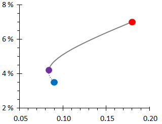
Figure 1: Real return as a function of volatility for various stock–bond portfolios. Blue: bonds, red: stocks, purple: minimum volatility (≈ 20% stocks).
In Figure 1, the curve indicates all possible stock–bond portfolios (from 100% bonds to 100% stocks). If one moves from the blue dot to the purple dot (that is to say if stocks are added to a bond investment) the return increases and the volatility decreases. The purple portfolio is therefore superior to the blue one in both respects. This is why the line is dotted: these are not portfolios one can reasonably choose.
Beyond the purple dot the return increases, but so does the volatility. It is then a matter of your circumstances and personal choice: more of both return and volatility, or less of both. The more cautious investors will be close to the purple dot, while the more daring will be towards the red dot. But investors between blue and purple dots, who probably consider themselves conservative, are in fact reckless. A portfolio with about one third of shares has the same volatility as a pure bond investment, but returns much more — this is a conservative investment.
How does it work? Stocks risk falling and losing money, but these falls do not usually happen when bonds fall (the latter being particularly sensitive to inflation). In the middle third of the figure below, for example, stocks rise and bonds fall slightly, in this case the purple portfolio rises a little. What will happen if stocks lose, say, 20%? In this case you will lose 20% of 20%, i.e. only 4%, which may be offset by a gain of the bond allocation. Thus, in Fig. 2 when the stock market falls by 30% the purple portfolio copes well. The purple portfolio returns a little more than the blue one (and much less than the red one) without high volatility (unlike the red one).
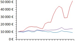
Figure 2: Purchasing power gains over 20 years on a (fictitious) investment of €10 000 in bonds (blue), shares (red) and 20% of shares (purple).
With two types of investments, returning respectively r1 and r2, the return of the portfolio is simply a weighted average: r = a r1 + (1−a) r2. However, the variance (the square of the volatility, i.e. of the standard deviation) is not a linear combination of the variances s12 and s22. Indeed, the variance is:
where p is the correlation between the two asset classes (between −1 and 1).
To minimise volatility, we take the first derivative of s2 with respect to a. We find a minimum at
This is the purple dot of Fig. 1.
If a fraction a of shares is added to a bond investment, since the standard deviation of stocks is twice as much as that of bonds, one gets a = (1 − 2p) / (5 − 4p), or a little less than 20% even with a slightly positive correlation. More specifically, if p ≈ 0, then to first order a ≈ (1 − 6p/5) / 5.
